The Oil Painting Filter

 ⇒ 

radius = 2 & intensity levels = 20

In this new tutorial, I will explain you how to apply the famous oil painting effect on an image. The function we will see is based on 2 important parameters : the radius and the number of levels of intensity. The radius simply defines how many pixels in each direction around the current one to look for, during the browsing of your image. For example, I used a radius of 2 to get the illustration above on the right. Concerning the number of levels of intensity, just note that the higher the value is, the more colorful the resulting image will be. I used the value 20 which is a good reference number.

The procedure :
Basically, each pixel will be put into an intensity "bin". The true intensity of a (Red,Green,Blue) pixel is defined as (Red+Green+Blue) / 3, and can range anywhere from 0 to 255. However, the oil paintings have a much more restricted effect, so each pixel will have its intensity binned.

❝ Data binning is a data pre-processing technique used to reduce [...]. The original data values which fall in a given small interval, a bin, are replaced by a value representative of that interval, often the central value. It is a form of quantization. ❞ (Wikipedia)

For each pixel, all pixels within the radius will have to be examined. Pixels within the radius of the current one are sub-pixels. For each sub-pixel, you must calculate the intensity, and determine which intensity bin that intensity number falls into. Maintain a counter for each intensity bin, which will count the number of sub-pixels which fall into each intensity bin. Also maintain the total Red, Green, and Blue values for each bin because these will be used to determine the final value of the pixel. After that, for each pixel, determine which intensity bin has the most number of pixels in it.

After we determine which intensity the pixel represents, as determined by the intensity bin with the most pixels, we can then determine the final color of the pixel by taking the total Red, Green, and Blue values in that specific bin, and dividing that by the total number of pixels in that specific intensity bin. As always, here is an understandable example of source code :

Let's finish this post with another example of the use of the oil painting filter :

This is not a random image.
It was scheduled for a tutorial on the human skin detection so I'll use it again when needed

⇓

radius = 2 & intensity levels = 20

до свидания!

Dithering

Dithering is used in computer graphics to create the illusion of "color depth" in images with a limited color palette - a technique also known as color quantization. In a dithered image, colors that are not available in the palette are approximated by a diffusion of colored pixels from within the available palette. The human eye perceives the diffusion as a mixture of the colors within it. Dithered images, particularly those with relatively few colors, can often be distinguished by a characteristic graininess or speckled appearance. For example, dithering might be used in order to display a photographic image containing millions of colors on a video hardware that is only capable of showing 256 colors at a time. The 256 available colors would be used to generate a dithered approximation of the original image. Without dithering, the colors in the original image might simply be "rounded off" to the closest available color, resulting in a new image that is a poor representation of the original. So I will try to present different methods designed to perform dithering...

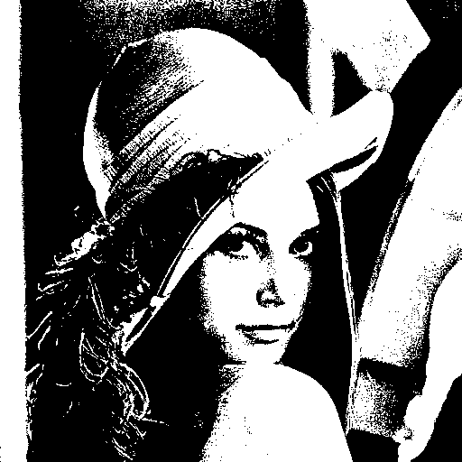
Thresholding :

"Averaging" grey level method used and n = 100

With the thresholding, you just have to convert your image in grey level with the method of your choice which explains the presence of the parameter style in the following source code example (here are the different methods we already saw) and then one pixel component value of every pixels (the Red, the Green or the Blue one because the grey level of a pixel always verifies Red=Green=Blue) must be compared against a fixed threshold n ranging from 0 to 255 that will determine the final color, Black or White. This may be the simplest dithering algorithm there is, but it results in immense loss of detail and contouring as you can see on my illustration above.


Random dithering :

"Averaging" grey level method used

Random dithering was the first attempt (at least as early as 1951) to remedy the drawbacks of thresholding. After converting your image in grey level, each pixel must be compared against a certain random threshold ranging from 0 to 255, resulting in a staticky image. Although this method doesn't generate patterned artifacts, the noise tends to swamp the detail of the image. It is analogous to the practice of mezzotinting.


Average dithering :

   

   

Average dithering is very similar to the thresholding method but this time, the threshold n at which all pixels are compared will depend on the image you want to process. It means that this threshold must be calculated from your input image and it is called the AOD (Average Optical Density). To get this value, convert your image in grey level, get the histogram of the resulting image (I assume you know how to create a histogram of the grey level which was explained here). Finally, the AOD is just the average intensity level of this histogram. The illustrations above show the result of the average dithering with the use of exactly 8 different grey level styles.

---

Floyd-Steinberg dithering :

"Averaging" grey level method used and n = 127

The Floyd-Steinberg algorithm (published in 1976 by Robert W. Floyd and Louis Steinberg), like many other dithering algorithms, is based on the use of error diffusion. This method works as follows. Each pixel in the original image is thresholded (as we saw with the thresholding method) and the difference between the original pixel value and the thresholded value is calculated. This is what we call the error value. This error value is then distributed to the neighboring pixels that haven’t been processed yet according to a certain diffusion filter :

The pixel indicated with a star (*) indicates the pixel currently being scanned, the blank pixels are the previously-scanned pixels, the pixels indicated with dots (...) are the pixels not affected by the error diffusion when processing the current pixel and the coefficients represent the proportion of the error value which is distributed (added) to the neighboring pixels of the current one.

Note that it exists an algorithm specially called the False Floyd-Steinberg algorithm providing poorer results and which can be applied with this diffusion filter where X is now the current pixel :

"Averaging" grey level method used and n = 127

         X   (3/8)
(3/8)  (1/4)  ...

Jarvis, Judice, and Ninke dithering :

"Averaging" grey level method used and n = 127

The Jarvis, Judice, and Ninke dithering (developed in 1976) is coarser, but has fewer visual artifacts. As you can see, the task is be a bit more fastidious. Indeed, the quantization error must now be transfered to exactly 12 neighboring pixels.

                  X     (7/48)  (5/48)
(1/16)  (5/48)  (7/48)  (5/48)  (1/16)
(1/48)  (1/16)  (5/48)  (1/16)  (1/48)

Stucki dithering  :

"Averaging" grey level method used and n = 127

The Stucki dithering (a rework of the Jarvis, Judice, and Ninke filter developed by P. Stucki in
1981) is slightly faster and its output tends to be clean and sharp.

                  X     (4/21)  (2/21)
(1/21)  (2/21)  (4/21)  (2/21)  (1/21)
(1/42)  (1/21)  (2/21)  (1/21)  (1/42)

Burkes dithering :

"Averaging" grey level method used and n = 127

Burkes dithering (developed by Daniel Burkes of TerraVision in 1988) is a simplified form of Stucki dithering that is faster, but is less clean than Stucki dithering.

                 X    (1/4)  (1/8)
(1/16)  (1/8)  (1/4)  (1/8)  (1/16)

Sierra dithering (the 3 existing) :

  

"Averaging" grey level method used and n = 127

Sierra dithering (developed by Franckie Sierra in 1989) is based on Jarvis dithering, but it's faster while giving similar results.

                  X     (5/32)  (3/32)
(1/16)  (1/8)   (5/32)  (1/8)   (1/16)
 ...    (1/16)  (3/32)  (1/16)   ...

Two-row Sierra is the above method, but was modified by Sierra to improve its speed.

                 X     (1/4)  (1/16)
(1/16)  (1/8)  (3/16)  (1/8)  (1/16)

Filter Lite is an algorithm by Sierra that is much simpler and faster than Floyd–Steinberg, while still yielding similar results (and according to Sierra, better).

         X   (1/2)
(1/4)  (1/4)  ...

Atkinson dithering :

"Averaging" grey level method used and n = 127

Atkinson dithering was developed by Apple programmer Bill Atkinson, and resembles Jarvis dithering and Sierra dithering, but it's faster. Another difference is that it doesn't diffuse the entire quantization error, but only three quarters. It tends to preserve detail well, but very light and dark areas may appear blown out.

         X    (1/8)  (1/8)
(1/8)  (1/8)  (1/8)   ...
 ...   (1/8)   ...    ...

---

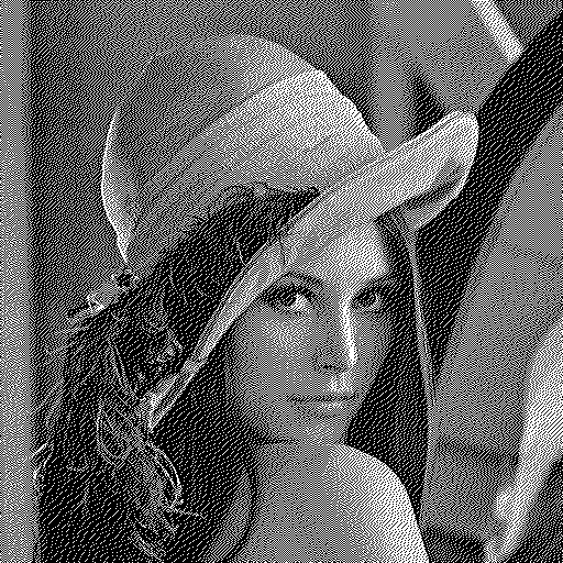
Ordered threshold :

Who is he/she?

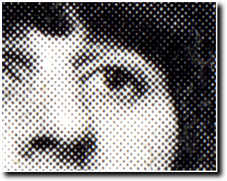
- Halftone effect with dots

 

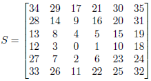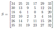
Note that the values of this threshold matrix are very low and  consequently this will change most of the pixels of your image into the white color if they are directly thresholded by each value of S as there is a bigger probability that your pixel values are higher than all these ones on a color scale ranging from 0 to 255 (unless your image is totally dark). 
So you must replace the values of S by (x * 255) / 35 where x is a value of this threshold matrix
(or else, each (y * 35) / 255 can also be simply thresholded by x where y is a pixel component value!)

With the ordered threshold method, instead of using a fixed threshold for the whole image (or random values for each pixel), a threshold matrix (named S here) of a predefined pattern is applied. The matrix paved over the image plane and each pixel of the image is thresholded by the corresponding value of the matrix. To apply the ordered threshold method, you must create a filter of the same size as your image by replicating the threshold matrix S on both directions as many times as possible (then by filling each extra columns/rows). It's the most difficult part of the processing because the dimensions of the threshold matrix S may or NOT divide the dimensions of your image. Finally, you just have to follow the thresholding method but with your new created filter. Note that I separately applied the thresholding method for each (Red,Green,Blue) pixel components so that the image is still in color (even if there are only 2³ types of color now as a pixel component value can be only 0 or 255). The threshold matrix S above can be used to obtain a halftone effect with dots (see illustration) and the get_dots function (line 2) just returns the threshold matrix S as it is defined.

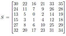
- Halftone effect with squares

This new threshold matrix S can be used to obtain a halftone effect with squares (see illustration) using again the ordered threshold method (like with all the following filters). The only differences to take in count are the new dimensions of S : 5x5 and its new values.

- Central white point

Same remark that the one previously evoked with the halftone effect

- Balanced centered point

Same remark that the one previously evoked with the halftone effect

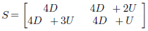
- Diagonal ordered matrix with balanced centered points

Same remark that the one previously evoked with the halftone effect but this time
the values of S₁ must be replaced by (x * 255) / 15 and the values of S₂ by (x * 255) / 31
where x is a value of S₁ or S₂.
(or else, each (y * 15) / 255 for S₁ or (y * 31) / 255 for S₂ can also be simply thresholded by x where y is a pixel component value)

- Dispersed dots or the Bayer filter

 

Same remark that the one previously evoked with the halftone effect

Hope  you  ❤  this   post!

Edge Detection

The new topic that we will see is closer to what we call "image processing" compared to what we already saw. Indeed, we will talk about the edge detection. It's the name used to describe a set of mathematical methods which aim at identifying points in a digital image at which the image brightness changes sharply or, more formally, has discontinuities. It exists many edge detection filters and I will present the most famous ones which always provide interesting results. Basically, the method used to apply these filters just consists in using certain convolution matrices (sometimes two at the same time for just one filter). I already explained the particularities of the convolution matrices and how to apply them on an image in this post. But let's reuse this previous understandable example :

On the left of the multiplication operator, there is the image matrix representation of the Green channel and on the right, there is a convolution matrix (also named kernel) with dimensions 3x3 and which is entirely filled with the value 0 except in one index containing the value 1. The result, where the value 42 circled in red appears, represents the new value that replaces the initial value 50 circled in red in the image matrix representation after applying the convolution matrice as follows :

new value = 40*0 + 42*1 + 46*0 + 46*0 + 50*0 + 55*0 + 52*0 + 56*0 + 58*0 = 42.

So we calculate the sum of products of the current pixel component and its 8 neighbors by the corresponding values, location based, in the convolution matrix (as a pixel has 3 channels : Red, Green and Blue, there are 3 sums to calculate). Note that in some cases, the new value must be divided by what we call a normalization factor as you will see. Now we can definitely start this new tutorial...

Prewitt filter :

The Prewitt operator is based on convolving the image with a small, separable, and integer valued filter in horizontal and vertical directions and is therefore relatively inexpensive in terms of computations. It was developed by Judith M. S. Prewitt. The convolution matrices' dimensions are 3x3 and have a normalization factor equal to 3 (like the Sobel filter). They must be filled with these following values :

Horizontal kernel

-1	-1	-1
0	0	0
1	1	1

Vertical kernel

-1	0	1
-1	0	1
-1	0	1

Sobel filter :

As you can see, the main difference with the Sobel filter is just the values of the convolution matrices. It was developped by Irwin Sobel who presented the idea of an "Isotropic 3x3 Image Gradient Operator" at a talk at the Stanford Artificial Intelligence Project (SAIL) in 1968.

Horizontal kernel

-1	0	1
-2	0	2
-1	0	1

Vertical kernel

-1	-2	-1
0	0	0
1	2	1

Roberts filter :

The Roberts filter was one of the first edge detectors and was initially proposed by Lawrence Roberts.

Normalization factor : 1 (like the Laplacian filter)

Horizontal kernel

0	0	0
0	-1	0
0	0	1

Vertical kernel

0	0	0
0	0	1
0	-1	0

Kirsch filter :

The Kirsch operator is a non-linear edge detector that finds the maximum edge strength in a few predetermined directions. It is named after the computer scientist Russell A. Kirsch.

Normalization factor : 15

Horizontal kernel

-3	-3	-3
-3	0	-3
5	5	5

Vertical kernel

-3	-3	5
-3	0	5
-3	-3	5

Laplacian filter :

The Laplacian of an image highlights regions of rapid intensity change and is therefore often used for edge detection (see zero crossing edge detectors). The Laplacian is often applied to an image that has first been smoothed with something approximating a Gaussian smoothing filter in order to reduce its sensitivity to noise (see my post on the blurring filters).

Horizontal kernel

0	-1	0
-1	4	-1
0	-1	0

Vertical kernel

-1	-1	-1
-1	8	-1
-1	-1	-1

The get_prewitt, get_sobel, get_roberts, get_kirsch and get_laplacian functions return 2 convolution matrices as they are respectively defined above. To see how they look like, look at the following get_high_pass function. Note that abs is the absolute value function (details).

High-pass filter :

  ⇒ 

The high-pass filter can be used to make an image appear sharper. This filter emphasizes fine details in the image – exactly the opposite of the low-pass filter. Unfortunately, while low-pass filtering smooths out noise, high-pass filtering does just the opposite: it amplifies noise. You can get away with this if the original image is not too noisy; otherwise the noise will overwhelm the image. High-pass filtering can also cause small, faint details to be greatly exaggerated. An over-processed image will look grainy and unnatural, and point sources will have dark donuts around them. So while high-pass filtering can often improve an image by sharpening detail, overdoing it can actually degrade the image quality significantly. To try this filter, you just have to apply a single convolution matrix (as I explained just before) with dimensions 3x3 and which must be filled with these values :

0	-1	0
-1	5	-1
0	-1	0

MDIF filter :

The last filter, which probably generate the best result, is the MDIF filter. Here again you will have to use two convolution matrices for an horizontal and then a vertical edge detection. These convolution matrices have the same dimensions : 5x5. And finally, the normalization factor is 12 and the convolution matrices must be filled with these values :

Horizontal kernel

0	-1	-1	-1	0
-1	-2	-3	-2	-1
0	0	0	0	0
1	2	3	2	1
0	1	1	1	0

Vertical kernel

0	-1	0	1	0
-1	-2	0	2	1
-1	-3	0	3	1
-1	-2	0	2	1
0	-1	0	1	0

The get_mdif function returns 2 convolution matrices as they are respectively defined above.

To finish, here is a last trick you can use to detect edges (without kernels) and at the same time, get the impression that your image is now a grey or white etching in relief like these 2 illustrations :

 

You must convert your image in grey level with the method of your choice (here are the methods we already saw). And as the grey level verifies Red=Green=Blue in each (Red,Green,Blue) pixel, let's assume that p0 is the Red or Green or Blue pixel component of the current pixel during the browsing of your image matrix representation and that p1, p2, p3, p4, p5, p6, p7, p8 are the 8 pixel components which surround p0 and of the same pixel channel. If you want to apply a grey etching for example, just replace the current pixel by (new value, new value, new value) where
new value = 8*p0 - p1 - p2 - p3 - p4 - p5 - p6 - p7 - p8 and then
new value = new value + 128 and finally new value = 255 - new value.

For the white etching this time, the two last steps are now : new value = fix_rgb(new value) and finally, new value = 255 - new value where fix_rgb is a function that checks if new value is correctly between 0 and 255 like all RGB pixel components values. That's all!