Image Transformations

In this new post, and after viewing some cool image distortions, we are going to see several useful image transformations like the horizontal and vertical flips, the rotation (of any pixel channel), the shifting (by wrapping an image around itself or not), the resizing (using the bilinear interpolation), the splitting, the shearing (which looks like a perspective view), the mipmapping and finally, I will present nearly all the existing mirror (reflection) effects.

Horizontal and vertical flips :

 

The horizontal and vertical flips are based on the famous swap function which consists in inverting the content of 2 elements. If you want to apply a horizontal flip for example, you will have to browse all the height of your image matrix representation and only the half of its width. In the first half of the width, for each row, each pixel will have to be swapped with its opposite pixel located in the 2^nd half of the width. The opposite pixel of the 1^st one on the 1^st row is the last one on this same row, ..., the opposite pixel of the n^th one is the (last one - n)^th one where n < (width/2). For the vertical flip, the principle is the same but you have to apply this procedure on each column this time and browse all the width of your image matrix representation and only the half of its height (see illustrations above).
Here is a function that can do the 2 flips according to the specified integer n :

Rotation :

   

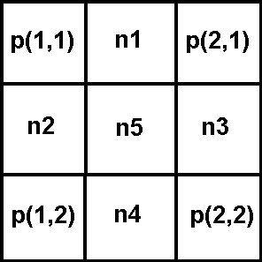
Now, if you want to rotate an image by an angle of n (n must be in radians, if n is in degrees, its radian value is (n*4*atan(1))/180 or (n*π)/180), you have to browse your image matrix representation and replace any pixel with coordinates (x,y) by the pixel located at (x',y') (only if x' and y' are inside the image matrix representation) where x' = cos(n)*(x - (width/2)) + sin(n)*(y - (height/2)) + (width/2) and y' = -sin(n)*(x - (width/2)) + cos(n)*(y - (height/2)) + (height/2).
Note that the rotation can be applied from another origin point than the middle of your image, you just have to change the parameters (width/2) and (height/2) in the given formulas and you can also rotate only certain pixel channels of your choice (see the 3 last illustrations).

Shifting :

 

The shifting of an image is nearly similar to the previous flips function. In fact, we don't invert the content of 2 elements but just erase one pixel by another. If you want to apply a horizontal shift to the right by a coefficient of xshift for example, you will have to browse your image matrix representation and on each row, the last pixel will have to be replaced by the (last one - xshift)^th one, ..., the (last one - n)^th pixel will have to be replaced by the (last one - n - xshift)^th one. Now, you have to do something with the surface which is not part of your resulting image. You can fill it with a color of your choice like on my illustration on the right or you can wrap your image around itself (left illustration). To wrap your image around itself, you firstly have to save the parts that will disappear due to the shifting, and after the shifting, you can finally display them at the correct location.

Resizing :

One of the famous methods used to increase the dimensions of an image is the bilinear interpolation. This method consists in creating a new surface bigger than the surface of your image, with dimensions (width*x)x(height*x) where x is a coefficient of your choice. Then you have to fill this new surface at every x pixels with the pixels of your image and calculate the values of the missing pixels (n1, n2, n3, n4, n5 on my illustration). If a missing pixel has exactly 2 known neighbor pixels, its value is the average of these 2 neighbors (n1 = (p(1,1)+p(2,1))/2, n2 = (p(1,1)+p(1,2))/2, n3 = (p(2,1)+p(2,2))/2 and n4 = (p(1,2)+p(2,2))/2) and if it is between 4 known neighbor pixels, its value is the average of these 4 neighbors (n5 = (p(1,1)+p(2,1)+p(1,2)+p(2,2))/4). Now, if you want to divide the width and the height of your image by a same value x, you can create a new surface with dimensions (width/x)x(height/x) and simply fill it with the pixels you will encounter at every x pixels on your original image. The 2 following resize_up and resize_down functions multiply/divide the dimensions of an image by a coefficient equal to 2 for example but the principle is similar for any other coefficient :

Splitting :

As we just saw the resize_down function which creates an image with dimensions equal to the original image ones divided by 2, the splitting function just consists in displaying 4 times the result of the resize_down function on a surface equal to the surface of your original image. Then you are free to continue to split the resulting image the number of time you want (details).

Actually, this transformation helped me to implement my Warhol filter which looks like that (this filter is intended to create an image similar to the tables of Andy Warhol who was an American artist and a leading figure in the visual art movement known as pop art) :

If you want to know how I got this result, you have to split your image, convert it in grey level with the method of your choice (here are the different methods we already saw), then you must posterize this grey level image, it means reduce the number of grey level colors. To do that and as you know the RGB colors go from 0 to 255, you can split this interval into ranges and during the browsing of the image matrix representation, you will have to check the grey level value of the current pixel and set its new grey level value among your reduced color palette (containing only Black, (96,96,96), (160,160,160) and White, for example) depending in which range the current value fall into:
0-64, 65-127, 128-191, 192-255.

At this point, your image should look like that :

Let's imagine that you considered 4 ranges like me during the posterization. You can then apply the following procedure to colorize your image : if the grey level value of the current pixel is in the 1^st range, the new color is Blue, in the 2^nd range, the new color is Magenta, in the 3^rd range, the new color is Yellow otherwise the new color is Orange. And as you see, I also applied a color rotation on the 4 thumbnails of Lena so that they are different but you can do all what you want concerning the number of splits, the number of ranges for the posterization, the choice of colors...

Shearing :

In plane geometry, a shear mapping is a linear map that displaces each point in fixed direction, by an amount proportional to its signed distance from a line that is parallel to that direction. In our case, what we will have to do is to move all pixels of an image with coordinates (x,y) to the location (x',y') where
x' = x + (xshift * y) - (width * xshift)/2 and y' = y + (yshift * x) - (height * yshift)/2.
Note that x', y' must be inside the image matrix representation and xshift, yshift are floating point numbers representing a horizontal and a vertical shifting coefficient of your choice between -1 and 1.

Mipmapping :

In 3D computer graphics, mipmaps (also MIP maps) are pre-calculated, optimized collections of images that accompany a main texture, intended to increase rendering speed and reduce aliasing artifacts. They are widely used in 3D computer games, flight simulators and other 3D imaging systems for texture filtering. Their use is known as mipmapping. Our goal here is to generate all the existing mipmaps of an image using the previous resize_down function and display them on a surface which has the same dimensions than the original image ones. If these dimensions are widthxheight, the dimensions of the first mipmap will be (width/2)x(height/2) (on the right of the illustration), ..., the dimensions of the n^th mipmap will be (width/2ⁿ)x(height/2ⁿ) where 2ⁿ < width.
Note that the way the mipmaps are displayed can obviously be changed (details).

Mirror effects :

   

   

As you see, it exists many mirror effects depending on the result you want to get (I named the 3^rd one "The Mussel"). The positive point is that the procedure to follow is always the same and is really easy. You have to get the half of an image in a matrix. It can be the right part, the left one, the top one or the bottom one. Now there are 2 possibilities of mirror effects. On one hand, the part you chose can remain identical and so you will have to replace the opposite part by the reverse of your selection using the previous flips function. On the other hand, the part you chose must replace the opposite part and be replaced by its reverse using again the flips function. Source code example :

Some Image Distortions & More

Because I know you ❤ the Mathematics (or not...), I suggest to show you several new image processing filters that can be applied using just a few mathematical functions that you may know and which are the cosine, the sine and the arctangent functions. Here are some details about them :

The Trigonometric Functions and The Inverse Trigonometric Functions.
Firstly, the image distortion will consist in changing the location of all the pixels (we won't have to change the color properties of the pixels like in my previous tutorials). But before moving any pixel to another location (which will have to be inside the image matrix representation), we obviously have to determine what will be the coordinates (x,y) of this new location. And it's here that the mathematical functions I just named will be useful concerning the filters that we will see. Finally, I will present the result of the use of different classic operators (+, -, *, ...) applied to 2 images.

Fisheye Lens effect :

The fisheye lens effect can give the impression that your image is zoomed and projected on a sphere (see the illustration). This effect is frequently used in photography. To get this result, you have to create a new empty image and fill it by seeking the pixels of the original image that are part of the sphere that you are creating. I can only suggest to refer yourself to this very well explained procedure (by Jussi) that I found by chance and which works perfectly. Note that in the following source code, sqrt is the square root function, atan is the arctangent function, cos and sin are respectively the cosine and sine functions and I manipulate some floating point numbers like with all the following distortion filters.

Polar effect :

The polar effect consists in converting the cartesian coordinates (x,y) of every pixels of your image matrix representation into polar coordinates. So this effect has as purpose to project your image on a circle (see the illustration). To get this result, you have to calculate the polar coordinates r (a radius) and φ (an angle in radians) where r = sqrt(x² + y²) and φ = 4*atan(y/x). Now, you can move every pixels to their new location (x',y') (only if x' and y' are inside the image matrix representation) where x' = r / 4 * cos(φ) + (image width/2) and y' = r / 4 * sin(φ) + (image height/2).

Wave effects :

  

Why wave effects and not wave effect? Because we will see exactly 3 types of wave : the horizontal and vertical ones and the combination of both. For the horizontal wave effect, each pixel with coordinates (x,y) must be replaced by the pixel located at (x',y) where x' = x + 20*sin(y * (2*4*atan(1))/128). Note that 4*atan(1) is a little trick I use to get exact value of π (3.141592653589793...) because atan(1) = π/4 so 4*atan(1) = π. For the vertical wave effect, the principle is similar, each pixel located at (x,y) must be replaced by the pixel located at (x,y') where y' = y + 20*sin(x * (2*4*atan(1))/128). The last wave effect can be obtained by replacing each pixel with coordinates (x,y) by the one located at (x',y'), it's just as easy as that. My waves function returns the desired effect according to the specified integer n :

Swirl effect :

The swirl effect is very similar to the polar effect. After calculating the polar coordinates

r = sqrt((x - image width/2)² + (y - image height/2)²) and φ =  r * (4*atan(1))/256 where (x,y) are the coordinates of the current pixel, this last one must be replaced by the pixel located at (x',y') where

x' = (x - width/2) * cos(φ) - (y - height/2) * sin(φ) + (width/2) and y' = (x - width/2) * sin(φ) + (y - height/2) * cos(φ) + (height/2). Note that this effect can be applied from another origin point than the middle of your image. You just have to change the parameters (image width/2) and (image height/2).

Ripple effect :

The ripple effect, like the swirl effect, can be applied at the origin point of your choice and you are free to set the number n of waves that will be generated and their amplification factor s. This time, after calculating the polar coordinates r = sqrt(x² + y²) and φ = atan(y/x) where (x,y) are the coordinates of the current pixel, this last one must be replaced by the pixel located at (x',y') where
x' = (r + (s * cos((r/R) * 4*atan(1) / 2*n))) * cos(φ),
y' = (r + (s * cos((r/R) * 4*atan(1) / 2*n))) * sin(φ) and R = sqrt((width/2)² + (height/2)²).

Warping effect :

The warping effect is probably the most disturbing distortion but actually, it can be useful for correcting image distortion or for the morphing which is a special effect that changes one image or shape into another through a seamless transition. To get the horizontal warping effect for example, you will have to replace any pixel with coordinates (x,y) by the pixel located at (x',y) where
x' = image width - (-sgn(x - (width/2)) / ((width/2) * (x - (width/2))² + (width/2))).
Sgn is the sign function (details). Here is a source code example :

---

According to plan, we will now see the use of some classic operators and their respective result using this image as the second test image :

So we have the image of Lena that we will name img1 and which contains a certain number of (Red1,Green1,Blue1) pixels, this new image, with the chameleon, that we will name img2 and which contains a certain number of (Red2,Green2,Blue2) pixels. Our goal is to create a new image that we will name img3.

Addition :

With this operation, the final image, img3, must contain (Red1+Red2, Green1+Green2, Blue1+Blue2) pixels. But you have to make sure that all sums result in values that are between 0 and 255.
Note that this rule must be applied to all the following functions.

Here is a source code example that will help to understand the following (I voluntarily created a third matrix, named matrix3, to well illustrate img1, img2 and the final result, img3 = img1 + img2) :

Subtraction left :

img3 must contain (Red1 - Red2, Green1 - Green2, Blue1 - Blue2) pixels.

Subtraction right :

img3 must contain (Red2 - Red1, Green2 - Green1, Blue2 - Blue1) pixels.

Difference :

img3 must contain (abs(Red1 - Red2), abs(Green1 - Green2), abs(Blue1 - Blue2)) pixels.

Note that abs is the absolute value function (details).

Average :

img3 must contain ((Red1+Red2) / 2, (Green1+Green2) / 2, (Blue1+Blue2) / 2)) pixels.

Multiplication :

img3 must contain
(255*(Red1/255 + Red2/255), 255*(Green1/255 + Green2/255), 255*(Blue1/255 + Blue2/255)) pixels. Note that in this case, you have to use floating point numbers when you are calculating x/255.

Cross Fading :

img3 must contain (Red1*f + Red2*f, Green1*f + Green2*f, Blue1*f + Blue2*f) pixels where f is a certain factor which must be between 0 and 1. The higher the value, the more brighter img3 will be. You can also choose different factors for each channel and here is a random idea, if you know how to horizontally or vertically flip an image (which is very easy), you can try to apply a cross fading effect between the original image and its reverse like that :

 

Amplitude :

img3 must contain
(sqrt(Red1² + Red2²)/sqrt 2, sqrt(Green1² + Green2²)/sqrt 2, sqrt(Blue1² + Blue2²)/sqrt 2) pixels.

Min :

img3 must contain (min(Red1,Red2), min(Green1,Green2), min(Blue1,Blue2)) pixels.

Max :

img3 must contain (max(Red1,Red2), max(Green1,Green2), max(Blue1,Blue2)) pixels.

...

It exists many other functions between 2 images like the boolean operations for example (AND, OR, XOR...) but the results were too terrifying! Apart from that, why not a bonus filter to finish this post? Have you ever heard about the anaglyphs? It's the name given to the stereoscopic 3D effect which allows you to see an image in 3D with your super stereoscopic glasses . To get this effect, it's very easy. When you have chosen an image (img1), you have to create a new image (img2) which corresponds to a horizontal shift of img1 (don't make a too big horizontal shift). Then you can create your anaglyph which has the particularity that all its Red pixel components must be the Red pixel components of img1 and all its Green and Blue pixel components must be the ones of img2.

Here is my result with a horizontal shift of 10px to the right :

¿ Cool ?

The Blurring Filters

Another interesting image processing topic... the blurring filters. As you may know, it exists many blurring methods simply because of the different types of result we want to get when we try to blur an image. For example, we generally use the pixelation when we want to anonymize a person or for censoring nudity. We can use the famous gaussian blur when we want to reduce the image noise and reduce detail. There is also a blurring filter named motion blur which can create a movement effect or lens blur which allows you to set the depth-of-field of the blur.

I found an article from Research at Google which talks about this last one :
Lens Blur in the new Google Camera app (by Carlos Hernández, Software Engineer).

So I think the blurring filters that I am going present will be the classic uniform blur, the pixelation, the Gaussian blur, the motion blur, the glass filter and an extra filter that we will name the progressive pixelation. I had the idea to try to implement this last filter when I found these images by chance :

 

Uniform blur :

n = 3

The uniform blur (also named the mean filter) is the easiest way to blur an image. The procedure to follow consists in replacing the pixels of your image by the average of the current pixel and the neighboring pixels during the browsing of your image matrix representation. So you will have to calculate the averages of the Red, Green and Blue pixel components of the current pixel and its 8 neighbors. I assume you know how to calculate an average so the only useful information I can give you is the following one. If the location of the current pixel on your image is (i,j), the locations of its 8 neighbors are

(i-1, j-1)	(i, j-1)	(i+1, j-1)
(i-1, j)	(i, j)	(i+1, j)
(i-1, j+1)	(i, j+1)	(i+1, j+1)

The most difficult part is to make sure the location of the neighbor pixel that you try to access isn't outside the image matrix representation (basically, this corresponds to the case of the image edges). One of the solutions that I decided to use is to browse the matrix from (1,1) to (width-2,height-2) and not from (0,0) to (width-1,height-1) where, in this case, my function would have try to access to pixel locations (-1,-1), ..., (width,height) which are out of bounds. Here is an example of source code :

This function takes an extra parameter n which determines the number of time this blurring method will be applied to an image. The higher the parameter n, the more intensive the uniform blur will be. Finally, as you may notice on my illustration, you can also try to blur only a certain region of your image with different forms like a circle, a rectangle, ...

Pixelation :

n = 16

The pixelation, like the uniform blur, is all about averaging but the procedure to follow is obviously different. Firstly, you will have to choose the size n of the future pixelated blocks.

Note that in my example, these blocks have a width and a height equal and that the size n should verify image width % n = 0 and image height % n = 0 (where % is the modulus operator) in order to have to same number of blocks horizontally and vertically (see the illustration). Then you have to browse your image matrix representation not pixel by pixel but block by block. And inside every blocks, all pixels must be replaced by the average of these same pixels. So you will have to browse every blocks one time to calculate the sums of the Red, Green and Blue pixel components and a second time to replace the pixels of each block by the final (Red,Green,Blue) values.

Here again, you can try to pixelate only a certain region of your image like a person's face.

Gaussian blur :

The Gaussian blur filter that I am going to present is based on the use of a kernel (more known under the name of convolution matrix). The convolution matrices can have different dimensions and the most important is the values they contain. Here is an example on how to apply a convolution matrix (on the right of the operator X) to an image matrix representation (note that in this case, the image matrix representation, on the left of the operator X, doesn't contain (Red,Green,Blue) values in each index but a single value. It's the matrix of the Green channel). The idea is to determine what is the value that will replace the current pixel component circled in red (50) if we apply the following convolution matrix. The answer is 42.

How we got this new value? Here is the method used :

new value = 40*0 + 42*1 + 46*0 + 46*0 + 50*0 + 55*0 + 52*0 + 56*0 + 58*0 = 42.

We calculate the sum of products of the current pixel component and its 8 neighbors by the corresponding values, location based, in the convolution matrix (as a pixel has 3 channels : Red, Green and Blue, there are 3 sums to calculate). In some cases, the new value must be divided by what we call a normalization factor as you will see. Now let's apply the convolution matrix of the Gaussian blur filter. The dimensions of this convolution matrix are 5x5, its normalization factor is 115 and it must be filled with these values :

2	4	5	4	2
4	9	12	9	4
5	12	15	12	5
4	9	12	9	4
2	4	5	4	2

The function can be written like that (note that like the uniform blur, you will have to find a solution for the case of the pixels which are on the image edges, these pixels haven't their 8 neighbors) :

Motion blur : Motion blur : Motion blur : Motion blur : Motion blur : Motion blur : Motion blur : Motion blur : Motion blur : Motion blur : Motion blur :

The motion blur filter is also the result of the use of a special convolution matrix. As you know what is a convolution matrix now, I can directly give you what you will need in order to apply this new filter but before, you just have to know that its particularity is that it can be applied with 3 different movement effects : "left to right", "right to left" and both at the same time. The dimensions of the convolution matrix are 9x9, its normalization factor is 9 and for the filling, it's very simple, put the value 0 everywhere except on the diagonal which goes from (0,0) to (8,8) and which must be filled with the value 1 for the "left to right" movement effect or the diagonal which goes from (8,0) to (0,8) for the "right to left" movement effect. Finally, the last movement effect is obtained by the combination of these 2 diagonals (this creates a X cross of 1 in the convolution matrix). I used the "left to right" movement effect :

Glass filter :

n = 4

The glass filter can create the same effect as your shower window which is probably opaque (see the illustration). And like the uniform blur, the function that I am going to present has an extra parameter n which determines the strengh of the opacity. To get this effect, you have to replace the pixels of your image by another pixel located at a random location within a certain fixed distance (3 in my example) so that the image remains distinguishable. Note that the get_random_neighbor function just returns a random value (corresponding to a horizontal/vertical random location) between values min and max.

Progressive pixelation :

n = 32

As we already saw the pixelation, the progressive pixelation function won't be difficult to implement. The idea is to choose a starting value which will correspond to the size n of the initial pixelated blocks. Note that here again, the initial pixelated blocks have a width and a height equal and that the size n should verify image width % n = 0 and image height % n = 0 (where % is the modulus operator) in order to have to same number of initial pixelated blocks horizontally and vertically. Then we will pixelate our image column by column using the previous pixelation function (each column has a width equal to n and a height equal to the image height) and at every x columns (x=3 in my example),  n  or rather a temporary copy of n will be divided by 2 and send to the pixelation function. The consequence is that it will create more smaller pixelated blocks at every x columns (see the illustration).

Finally, here is the last example of source code :

Next time, we will do some mathematics.